I’ve been streamlining legacy data sets the past week or so, such as daily min/max temperatures recorded on Tumamoc Hill from roughly 1906 to 1995, but with a lot of missing data, and some errors caused by faulty readings. If it were a complete set of daily readings over that time, it would be more than 32,000 records. But due to lots of missing data and errors, it’s about half that.

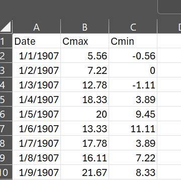
In Excel, it looks like the above. Reading this csv file into R is easy enough. But I realized that a set of daily temperatures over almost a century is of limited value for saguaro cactus ecology, which is what we are working on. So I wanted to change the temporal scale of the data to weekly and/or monthly. Especially using monthly data, it’s useful to aggregate that into seasons, such as the warmest quarter of the year and the coldest quarter of the year, and see if those seasonal cycles say anything about our saguaro habitat.

Working with this data in R poses a few challenges. The first is that the Date column is a character string, not recognized as dates by R. So you have to convert the entries in that column into the class of data in R that is readable as a date. It used to take me forever to figure out how to do that, but I’ve got that workflow down fairly reliably. The package “lubridate,” which is part of the tidyverse, handles date conversions and formatting very well. It’s a single line of code:

Dates <- mdy(climatedata$Date)

Then you can easily add this to your data frame and remove the original Date column:

climatedata<-climatedata%>%mutate(Dates=Dates)
climatedata <- climatedata %>% select(-Date)

Having done that, I was wondering how to generate monthly and weekly statistics from these thousands of daily temperatures, and I thought I would have to write my own function, and run it in a repeating piece of code called a “for loop.” I am not very good at that. But on the off chance that there was an easier way, I searched “generating weekly or monthly data from daily data,” and lo and behold, good old lubridate and another package within the tidyverse can do it in two lines of code. From lubridate, you can select which temporal span you want, for example:

climatedata$week <- floor_date(climatedata$Dates, “week”)

And then you can use the summarize pipeline from dplyr, for example for weekly means of both the min and max temps:

dmin<-climatedata %>%
group_by(week) %>%
summarize(min = min(Cmin))

dmax<-climatedata %>%group_by(week) %>%
summarize(max = max(Cmax))

This works for monthly means, or other summary statistics such as the weekly or monthly minima or maxima.

I don’t know about you, but for me, nothing is as much of a relief (at least in my research life) as finding a functioning, repeatable work flow for data management and analysis that runs successfully in R. I have been working in R for about 11 years, and it still throws me curveballs. But the quality of online help and quick solutions has really gone up over that time.

By the way, the featured image for this post is one of my favorite taquerias, anywhere, the amazing Taqueria Pico de Gallo in South Tucson. A car crashed into the building a few years ago but they kept selling tacos outside. I hope they’ve been able to fic the place up.

Above, a dying saguaro on the south plot of Tumamoc Hill, during our survey in 2023. One of the aspects of saguaros that is intriguing is that the mortality rate stays relative constant over many different time periods with different climate conditions. However, in parts of the range, elevated mortality is appearing, as a response to heat and drought. With our Tumamoc population, we want to see if we can pick up a signal of changes in mortality, or changes in which part of the population is more likely to die. And for that, we will probably need the above legacy temperature data.