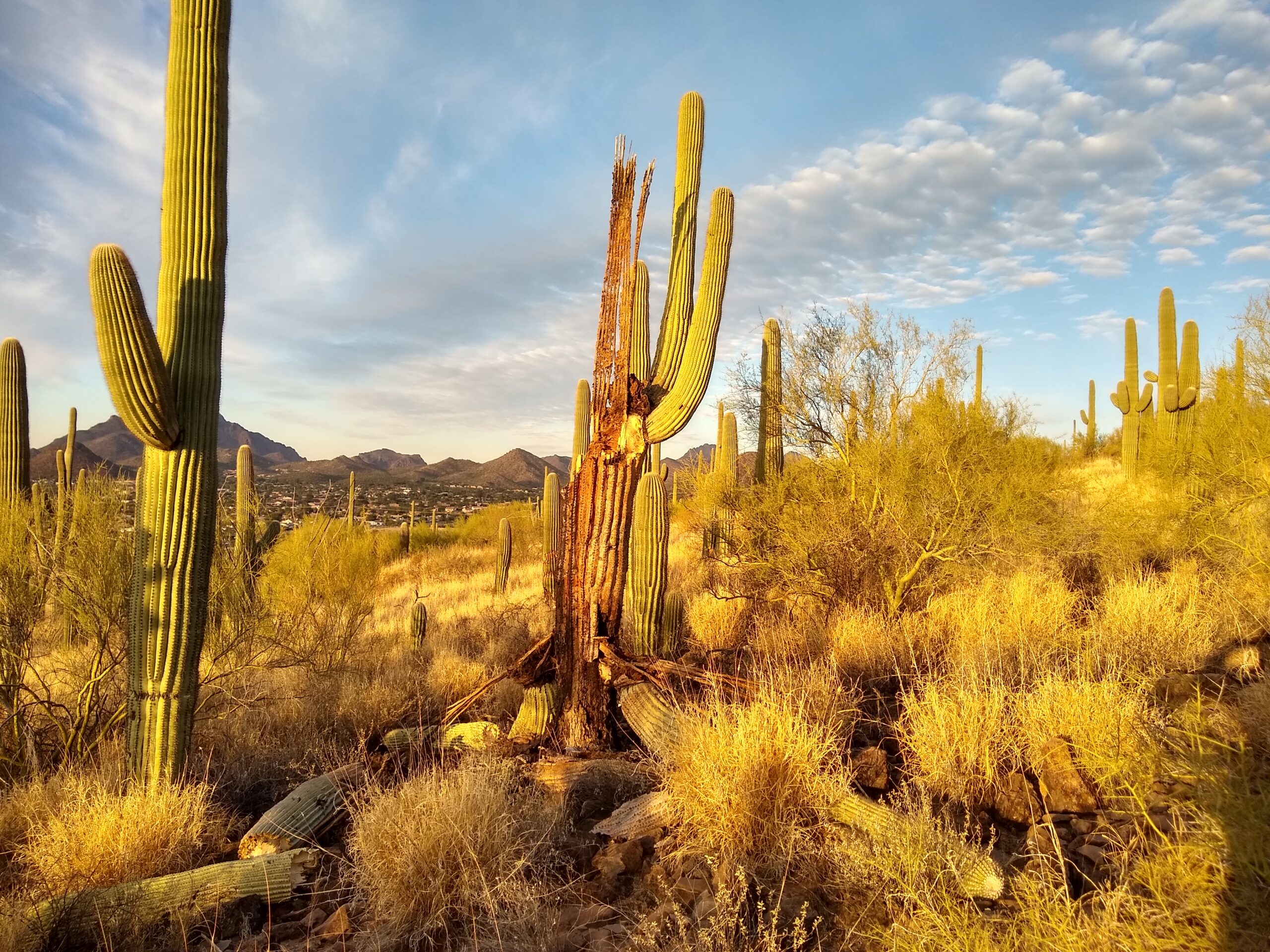
Not paralysis if you have all the time in the world. But who has all the time in the world? It’d be a lot cooler if we did.

In this case, I’m referring to the regression models used to parameterize an integral projection model (IPM).

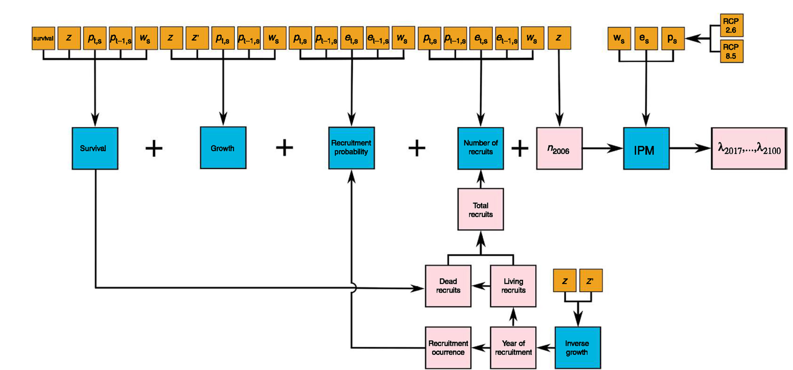
The above is a schematic diagram for steps involved in developing an integral projection model, which is a type of model used to understand current and future population dynamics. Across the top (orange boxes) are the environmental variables used in regression models to create a best model for how those variables affect survival or growth rate over time. The complex set of steps for recruitment probability on the right use an inverse growth model and the survival and growth parameters to estimate recruitment. All of these parameters are then deployed in the actual IPM, with two projections (in this case) using predicted climate chnages under two representative concentration pathways: RCP 2.6 (best case) and 8.5 (worst case) between the present and 2100. Diagram from Félix-Burruel et al. 2025.

My current project is to develop an IPM for the saguaro cactus population on Tumamoc Hill in Tucson. We have repeat survey data at roughly 10-year intervals from 1964 to 2022, with the last survey including microsite conditions around each saguaro. Since IPMs require evenly spaced time between transitions, we used six-year intervals and interpolated the height of the main stem of each saguaro, creating ten approximately six year intervals: 1964, 1970, 1976, 1982, 1987, 1993, 2000, 2006, 2012, 2017, and 2022. The years in bold are actual survey years, with interpolation years not in bold. This gave us 10 transitions.

It took several months to generate our interpolated height data, before even starting the entire IPM process. The interpolation of heights for transitions that were not from actual survey data required a complex forward and backward regression process. We had several false starts and had to go back to the beginning repeatedly, mostly because we had 60 years of complex data involving several different “kinds” of saguaro events between actual surveys (“disappearing” saguaros that were measured once and never measured again, “zombie” saguaros that were measured in one survey, missing from the next one, and then reappeared in the one after that, “negative height” saguaros that were decapitated or perhaps measured in error, so that their change in height was negative in the later survey, and pesky duplicate ID numbers that created havoc). We started the process of preparing the transition data and interpolated heights in April 2025, and the data was not in good shape until September. Huge, old, complex, legacy data sets need a lot of attention, a lot of care, and a lot of adjustments. Since the continuous variable of the height of the main stem of each individual saguaro, combined with accurate mortality and recruitment data, were the essentials for the IPM, this detailed attention was absolutely not optional.

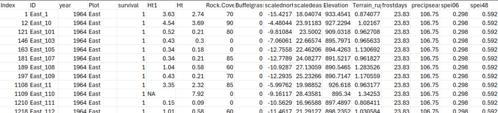
The below is the first 11 lines of our 6000-row final data frame. You might notice that our sitewide climate data starting with frost days have fixed values for each year (1964 in this case), as we had to use six-year running averages of this climate data, to match the temporal scale of our transitions (10 transitions at six years each). A limitation, but unavoidable since we do not currently have microclimate data for each saguaro. Survival from 1964 to 1970 is coded with either a 1 or a 0. Ht1 is the height in 1970; Ht is the height in 1964. From the 10 variables for each saguaro, we selected seven.

My colleagues and I launched the regression models for all combinations of between one and six variables as fixed effects, and the year as a random effect; mostly environmental variables from microsites at a 0.78 sq. m scale around each saguaro (cf. Breslin et al. 2025), but also sitewide climate data. For the survival model: buffelgrass percent cover, aspect (as slope aspect times slope angle, per Stage 1976), elevation, frost days (number of days below 0 C), precipitation seasonality (the coefficient of variation of precipitation for the year), and standardized precipitation evapotranspiration index with 4-year rolling averages, with survival as the response and year as the random effect (alone and in interation with each fixed effect); for the growth model, we used a slightly different set of variables, using terrain ruggedness instead of precipitation seasonality, with size at the next year as the response, and year plus all possible interactions as the random effect. These variables were assigned to more than 6000 saguaros over the entire period from 1964 to 2022.

My colleagues were co-authors on Félix-Burruel et al. 2025, and they mentioned that their methods had been repeatedly revised due to reviewer feedback and multiple rounds of revision, so I enthusiatically agreed to follow their methods for the paper that did get published. Their approach is to perform regressions using all possible combinations of variables in an exhaustive, multi-model approach, calculating the average root mean squared error (RMSE) for each model, with each possible configuration iterated 30 times. The R code for both survival and growth regression model runs is 650 lines long.

We began running the R code for these regressions for survival and growth in late November, but had some errors and false starts, and adjusted a few times, finally disaggregating and running all configurations separately on a dedicated gpu at the University of Arizona. The learning curve was pretty steep for me getting R code to run on this remote machine, since I first had to create an R environment specific to this project, and then launch several dozen tmux windows each with a different model configuration running. Of course, the single variable up to four variable models for both survival and growth ran much more quickly (we ran those on the high performance cluster at U of A). Those jobs started in earnest after some adjustments, on December 26, 2025, and finished on February 3, 2026. This process involved submitting more than 60 batch scripts, using different R code for each, and tracking the csv files to which results were written, and waiting for these csv files to not have any more data written to them.

Many of the five and six variable configurations are still running, more than 3.5 months later. As variables are added to these regression models, the possible configurations and interactions increase exponentially, and each model runs much more slowly. One good thing is that any model configuration where any two terms are > 70% correlated does not run. For example, this threshhold was reached in every possible seven variable model, so those won’t be included.

The below is what it looks like when I navigate to the remote gpu and “attach” a tmux session. Tmux is great because you can run multiple jobs simultaneously, and when you attach a particular session, it just looks like it is running on your own machine.

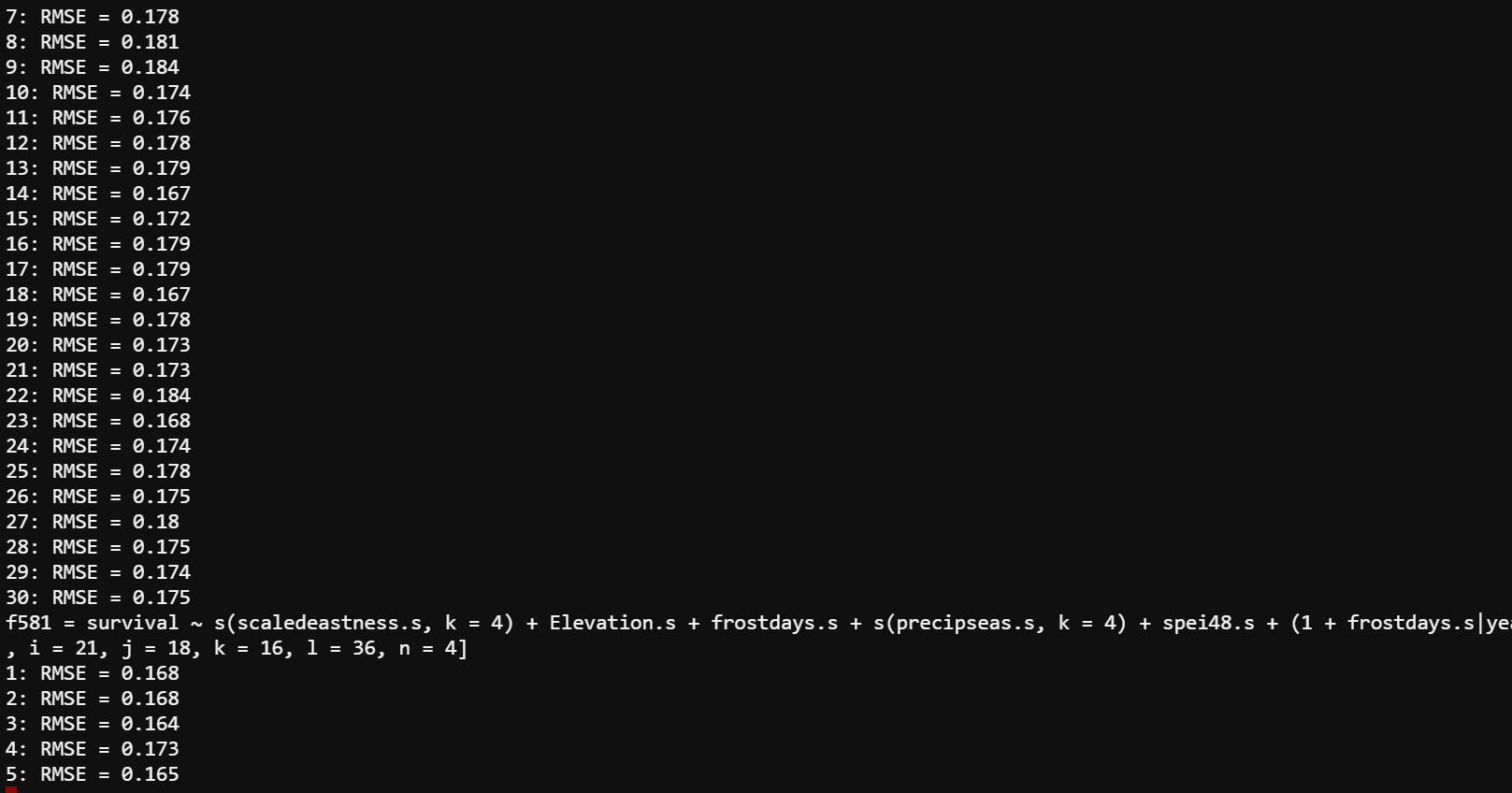
Here’s an example generalized additive mixed model for survival, from a five-variable set of configurations that is still running, copied from the view within the tmux window on the gpu:

f658 = survival ~ s(Buffelgrass_Cover.s, k = 4) + scaledeastness.s + s(frostdays.s, k = 4) + s(precipseas.s, k = 4) + s(spei48.s, k = 4) + (1 + frostdays.s|year) [df = 735, n.f = 5, i = 19, j = 23, k = 16, l = 36, n = 16]
1: RMSE = 0.17
2: RMSE = 0.166
3: RMSE = 0.164
4: RMSE = 0.173
5: RMSE = 0.166
6: RMSE = 0.164
7: RMSE = 0.169
8: RMSE = 0.171
9: RMSE = 0.173
10: RMSE = 0.163
11: RMSE = 0.168
12: RMSE = 0.171
13: RMSE = 0.17
14: RMSE = 0.157

After 16 more iterations, this particular configuration will generate an average RMSE, and the algorithm will move on to the next configuration. This is the 658th configuration for this subset of possible configurations of five variables plus random effects and interaction terms. This configuration set might be close to done, as a similar set ended after 650 models iterated 30 times (19,500 five-variable model iterations total). However, some configuration sets go through 2000 or more possible combos, with 30 iterations each, for more than 60,000 model iterations. By the way, the actual average RMSE is calculated with extreme precision, such as 0.162490177820578, to the nearest tenth of a quadrillionth. The rounded values are shown in the example above. This is because the differences in RMSE are often quite small, and yet the comprehensive model selection requires that those small distinctions be measured.

A test run of a faster than average five-variable configuration set performed 30 iterations per configuration in 50 minutes. Consequently, if there are about 700 different possible configurations that pass the correlation threshhold, that configuration set will take about a month of high-speed computing days. Six variable models are much slower. A six variable model we started on the gpu on January 17, 2026, has completed 375 model configurations, out of maybe 1000 total, for a possible exhaustive run time of 237 days, fully completing somewhere around the middle of September.

In theory, this exhaustive approach should provide the best survival model, and the best growth model, as selected based on root mean squared error. The best survival and growth models are then used in the complex inverse growth model that is used to create the recruitment kernel for the IPM, after which the IPM can finally be run under projected climate scenarios.

Here’s the thing: different people are on different imagined timelines with this project. My colleagues with the expertise in the modeling process want the exhaustive process to run in full. My supervisors on the project wish it were submitted for publication already. I can see the perspective of both of these imagined timelines.

On the one hand, what’s the hurry? We are not under a deadline. I always finish projects whether I am getting paid or not, regardless of what other projects come up (paid or not). A molecular phylogenomic study of Caribbean cacti including estimates of ancestral biogeography was handed off to me as a “side project” with me as lead author in July, 2024. The co-authors and I are finally at the full draft stage, this month. Some of the analyses for that paper took more than eight months, mostly for multimodel comparison for the strongest inference.

On the other hand, I know there are other researchers who simply never finish stuff like this. This has never been the case for me, but my supervisors are concerned that this saguaro IPM paper will just never be completed. I get it. Models that run for nearly a year seem like they will never stop. The exhaustive modeling process that we launched in December is, however, finite.

I’m at a crossroads where I think the best approach now is to use all of the results we currently have, proceed, run the recruitment models as quickly as possible, and get some IPM results. We can do all of these next steps while the exhaustive modeling just continues in the background. My last paper was submitted in December, 2024, and not published until June 2025. Seven months between submission and re-submission, and acceptance. This kind of publishing timeline (which is actually somewhat on the fast side) gives us plenty of time to let the models run, and do some quick comparisons in the revisions stage.

I honestly don’t know though. Part of me has the mindset: “Do I want this done soon, or do I want it done right?” Perhaps there is a middle ground, with “good enough” models, but it also seems a shame to start a process that is meant to be exhaustive and cut it short, after three months. However, of course, it won’t hurt to go with what we have, get some results, and see.

In many areas now in quantitative analysis, complex approaches have been made possible by exponentially increased computational resources. Many of these complex approaches provide much stronger inference, and more insight into covariates that affect plants.

My colleagues and I are talking about ways to streamline the code so it runs faster in R, and perhaps introducing a penalized likelihood or Bayesian criterion to more aggressively filter possible models, reducing the entire model space. I was “raised” in Caswellian discrete matrix population models, and I have been doing a separate analysis using discrete life stages of the saguaro and looking at patterns over time and space. I think there’s room for all kinds of approaches based on the data, the organism, and the environmental biology.